In short ⚡
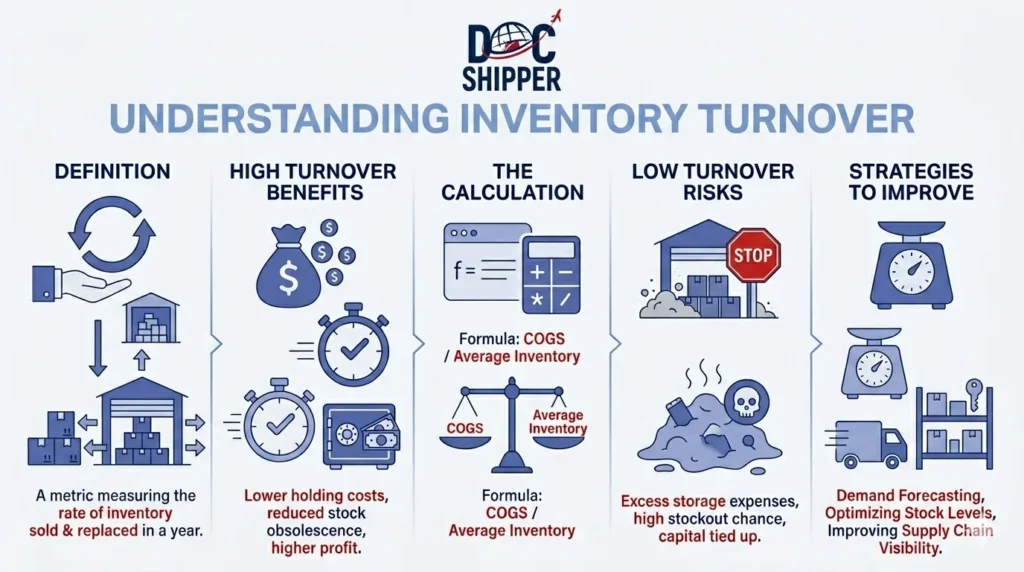
Inventory Turnover is a financial ratio measuring how many times a company sells and replaces its stock within a specific period. It indicates inventory management efficiency and reveals how quickly products move through the supply chain, directly impacting cash flow and warehouse costs in international trade operations.
Introduction
Many importers struggle with the same critical dilemma: Should they order large shipments to reduce unit costs, or maintain lean inventory to preserve cash flow? This tension between procurement strategy and working capital management becomes particularly acute in international logistics, where lead times stretch across weeks or months.
Inventory turnover provides the answer. This metric reveals whether your stock moves efficiently or sits dormant, accumulating storage fees and tying up capital. For businesses engaged in cross-border trade, understanding turnover rates becomes essential to optimizing order quantities, warehouse selection, and supplier negotiations.
Key characteristics of inventory turnover include:
- Performance indicator: Measures operational efficiency in converting inventory to sales
- Cash flow impact: Higher turnover typically means faster capital recovery
- Industry-specific: Optimal rates vary dramatically between perishable goods and durable products
- Strategic tool: Informs decisions on order frequency, MOQ negotiations, and warehouse sizing
- Risk signal: Low turnover may indicate overstocking, obsolescence, or demand miscalculation
Technical Breakdown & Strategic Implications
The standard calculation divides the Cost of Goods Sold (COGS) by Average Inventory Value. The formula expressed: Inventory Turnover = COGS ÷ ((Beginning Inventory + Ending Inventory) ÷ 2). This produces an annualized ratio showing how many complete inventory cycles occurred during the measurement period.
Understanding the inventory holding period provides complementary insight. Calculate this by dividing 365 days by your turnover ratio. A turnover of 6 means inventory sits an average of 61 days before sale. For importers, this metric must account for international transit times, customs clearance delays, and seasonal demand fluctuations.
The working capital implications extend beyond simple storage costs. Each day products remain unsold represents locked capital that cannot fund new purchases, marketing initiatives, or business expansion. Companies with annual turnovers below 4 often face liquidity constraints, particularly when managing letters of credit or prepayment terms common in international trade.
Industry benchmarks vary significantly. Perishable goods sectors like fresh produce may achieve turnover rates of 50-100, while luxury furniture retailers might operate efficiently at 3-5. According to U.S. Census Bureau data, wholesale trade inventory turnover averages 7.2 annually, though this masks substantial variation across product categories.
The relationship between turnover and supply chain configuration proves critical for international operations. Higher turnover rates demand more frequent shipments, potentially increasing per-unit transportation costs while reducing warehousing expenses. At DocShipper, we help clients model these trade-offs, determining whether consolidated monthly ocean shipments or weekly air freight better aligns with their turnover objectives and margin structures.
Optimizing turnover requires balancing five competing priorities: maintaining sufficient safety stock to prevent stockouts, minimizing capital tied up in inventory, securing volume discounts through larger orders, reducing per-unit logistics costs, and accommodating lead time variability inherent in international shipping. The optimal turnover rate emerges from this multi-variable equation rather than pursuing the highest possible number.
Practical Examples & Performance Data
Consider two importers of consumer electronics from China, each generating $1.2 million in annual COGS. Company A maintains $400,000 average inventory, achieving a turnover of 3. Company B operates with $150,000 average inventory, turning over 8 times annually.
| Metric | Company A (Turnover: 3) | Company B (Turnover: 8) |
|---|---|---|
| Average Inventory | $400,000 | $150,000 |
| Days Inventory Held | 122 days | 46 days |
| Annual Warehouse Cost (8% of inventory value) | $32,000 | $12,000 |
| Opportunity Cost (10% annual capital cost) | $40,000 | $15,000 |
| Shipment Frequency | Quarterly (4x/year) | Every 6 weeks (8x/year) |
Company B saves $45,000 annually in combined holding and opportunity costs. However, their frequent shipment model increases logistics complexity and per-unit freight expenses. The net advantage depends on whether increased shipping costs exceed the $45,000 savings, which varies by product density, container utilization, and incobound routing options.
Seasonal variation analysis: A fashion importer experiences turnover fluctuations from 12 during peak season (September-December) to 3 during slow months (February-April). Rather than using the annual average of 6.5, sophisticated inventory planning segments turnover by quarter, adjusting order quantities to match demand velocity and prevent both stockouts during peaks and excess inventory during troughs.
SKU-level optimization: An industrial equipment distributor stocks 500 SKUs with vastly different turnover profiles. The top 20% of products turn over 15 times annually, while the bottom 30% achieve only 1.5. By applying ABC analysis—concentrating working capital on high-turnover items and implementing make-to-order strategies for slow movers—they improved overall turnover from 4.2 to 6.8 while reducing stockouts by 35%.
Multi-country warehouse strategy: A company importing from Vietnam to serve European markets compared centralized warehousing in Rotterdam (turnover: 5.5) versus distributed inventory across Germany, France, and UK (combined turnover: 8.2). The distributed model required 30% more total inventory but reduced last-mile delivery times from 5 days to 2 days, improving customer retention sufficiently to justify the lower turnover efficiency.
Impact of payment terms: When negotiating with Asian suppliers, a retailer shifted from 30% deposit/70% on shipment to 100% payment after 60-day credit terms. This adjustment allowed them to receive and sell products before payment was due, effectively improving cash-adjusted turnover from 6 to infinity during the credit period, though the supplier added a 3% price premium that still yielded net positive economics.
Conclusion
Inventory turnover serves as the critical metric connecting procurement strategy, logistics execution, and financial performance in international trade. Optimizing this ratio requires balancing capital efficiency against operational complexity while accounting for industry norms and supply chain constraints specific to cross-border commerce.
Need assistance optimizing your inventory strategy across international supply chains? Our experts at DocShipper analyze your turnover metrics, lead times, and cost structures to design efficient procurement and warehousing solutions. Contact us to transform your inventory management approach.
📚 Quiz
Test Your Knowledge: Inventory Turnover
What does inventory turnover fundamentally measure?
A company achieves an inventory turnover of 12. What is the correct interpretation?
An importer ships from Asia with 45-day ocean freight lead times. Which strategy best applies inventory turnover principles?
🎯 Your Result
📞 Free Personalized QuoteFAQ | Inventory Turnover: Definition, Calculation & Concrete Examples
No universal "good" ratio exists—optimal turnover depends entirely on your industry, product type, and business model. Grocery retailers might target 15-20, while industrial machinery distributors operate efficiently at 3-5. Compare your performance against direct competitors and industry benchmarks rather than absolute numbers. Excessively high turnover may indicate stockouts and lost sales opportunities, while very low ratios suggest overstocking or obsolescence risks.
These metrics represent inverse perspectives on the same concept. Inventory turnover measures how many complete cycles occur annually (COGS ÷ Average Inventory), while inventory days calculates the average time products remain in stock (365 ÷ Turnover Ratio). A turnover of 12 equals 30 inventory days. Days provide more intuitive understanding for operational planning, while turnover ratios facilitate benchmarking and financial analysis.
COGS provides the accurate method since both numerator and denominator use cost basis, enabling apples-to-apples comparison. Using sales revenue in the numerator while inventory remains at cost basis creates distortion from markup percentages. Some analysts use revenue-based calculations for quick approximations or when COGS data is unavailable, but this approach compromises precision and comparability across companies with different margin structures.
Extended lead times from Asia or other distant origins force lower optimal turnover rates due to required safety stock buffers. A domestic supplier with 5-day replenishment enables much higher turnover than a 45-day ocean freight supply chain. Calculate your reorder point as (daily sales rate × lead time in days) + safety stock, then model how different order frequencies impact both turnover ratios and stockout risks before committing to aggressive targets.
Yes—pursuing turnover optimization without considering trade-offs creates multiple risks. Ordering smaller quantities more frequently increases per-unit shipping costs and administrative burden. Reducing safety stock to boost turnover raises stockout probability during demand spikes or supply disruptions. The optimal strategy balances turnover efficiency against service levels, procurement costs, and operational complexity rather than maximizing the ratio itself.
Annual turnover ratios mask seasonal businesses' true performance. Calculate separate turnover rates for peak and off-peak periods, then use weighted averages based on period duration. For highly seasonal items like holiday decorations or summer sports equipment, consider measuring turnover only during active selling seasons, excluding off-season holding periods when minimal movement is expected and planned.
Use the same inventory valuation method (FIFO, LIFO, or weighted average) consistently in both COGS and inventory balance calculations. FIFO generally produces slightly higher turnover ratios in inflationary environments since older, lower-cost inventory appears in COGS while newer, higher-cost inventory sits on the balance sheet. Consistency matters more than method choice for trend analysis and internal benchmarking.
Technology products, fashion items, and other goods with high obsolescence risk require significantly higher turnover targets—often 10-20 or above—to minimize markdown losses from outdated inventory. Commodity products with stable demand and no expiration concerns can operate efficiently at lower turnover rates. Align your target turnover with product lifecycle characteristics rather than applying uniform benchmarks across diverse SKU portfolios.
Both metrics provide valuable but different insights. Total inventory turnover reveals overall working capital efficiency and guides aggregate financial planning. SKU-level analysis identifies slow-moving products that drag down performance and fast-movers deserving increased inventory allocation. Sophisticated operations segment inventory into A/B/C categories, applying different turnover targets and management strategies to each tier based on sales velocity and strategic importance.
Five primary levers exist: negotiate shorter supplier lead times enabling smaller, more frequent orders; improve demand forecasting accuracy to right-size safety stock; implement just-in-time or vendor-managed inventory programs; eliminate slow-moving SKUs through product line rationalization; and leverage technology like automated reorder point systems that respond dynamically to actual sales velocity rather than static forecasts.
Warehouse proximity to customers enables faster replenishment cycles and lower safety stock requirements, supporting higher turnover. A centralized facility 1,000 miles from your market might require 15 days of safety stock for a 95% service level, while a local warehouse needs only 5 days. However, distributed inventory across multiple regional facilities typically reduces individual location turnover even as it improves service levels—requiring total system analysis rather than single-warehouse metrics.
Initial improvements often appear within one inventory cycle (365 ÷ current turnover ratio). A company with turnover of 6 should see measurable changes within 60 days of implementing new policies. However, sustainable optimization requires 3-4 complete cycles to fully validate new ordering patterns, safety stock levels, and supplier relationships. Resist judging initiatives prematurely—temporary disruptions during transition periods often precede long-term gains.
Need Help with
Logistics or Sourcing ?
First, we secure the right products from the right suppliers at the right price by managing the sourcing process from start to finish. Then, we simplify your shipping experience - from pickup to final delivery - ensuring any product, anywhere, is delivered at highly competitive prices.


Fill the Form
Prefer email? Send us your inquiry, and we’ll get back to you as soon as possible.
Contact us 

