In short ⚡
Forecasting is the analytical process of predicting future demand, supply chain requirements, and logistics capacity based on historical data, market trends, and statistical models. In international trade, accurate forecasting determines inventory levels, shipping schedules, warehouse allocation, and procurement strategies—directly impacting cost efficiency and customer satisfaction.
Introduction
How many containers should you book for Q4? When will your warehouse reach maximum capacity? These questions plague import/export managers daily. Without forecasting, businesses face either stockouts that lose sales or overstocking that drains working capital.
In global supply chains, forecasting bridges the gap between volatile consumer demand and fixed logistics infrastructure. It informs procurement cycles, shipping frequencies, and customs clearance planning—ensuring goods arrive precisely when needed, not weeks too early or catastrophically late.
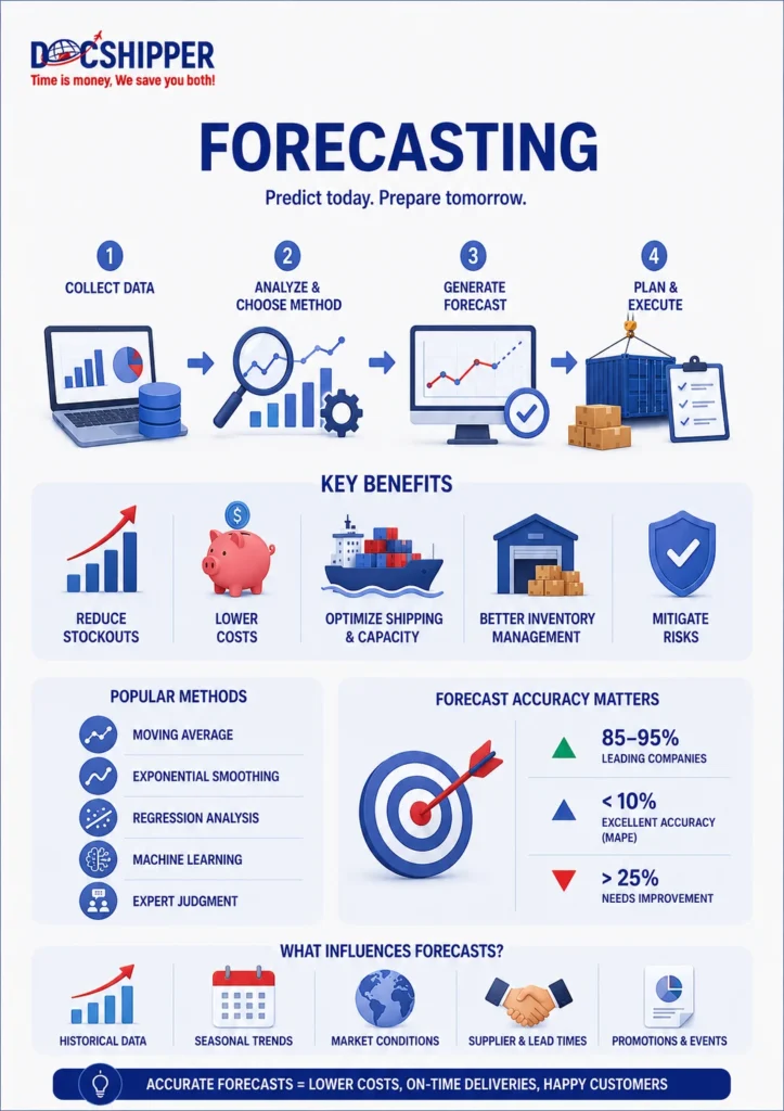
Key characteristics of effective forecasting include:
- Quantitative rigor: Statistical models (moving averages, exponential smoothing, regression analysis)
- Qualitative judgment: Market intelligence, seasonal trends, promotional calendars
- Continuous refinement: Feedback loops comparing forecasts to actual outcomes
- Cross-functional collaboration: Sales, operations, and finance alignment
- Technology integration: ERP systems, AI-driven predictive analytics, demand sensing tools
Forecasting Methods & Strategic Application
Modern logistics forecasting combines time-series analysis with real-time market signals. The most common methods include moving averages for stable demand patterns, exponential smoothing to emphasize recent data, and causal models linking demand to external variables like GDP growth or competitor pricing.
For seasonal businesses—think toys before Christmas or electronics during Black Friday—seasonal decomposition models separate trend, seasonality, and irregular components. This precision prevents the costly mistake of applying last year’s February data to predict December volumes.
Collaborative Planning, Forecasting, and Replenishment (CPFR) represents the gold standard in supply chain forecasting. Trading partners share point-of-sale data, promotional schedules, and inventory positions to create a single, synchronized forecast. According to GS1 standards, CPFR implementations reduce forecast error by 20-40% compared to siloed approaches.
Machine learning now elevates forecasting beyond traditional statistics. Neural networks detect non-linear demand patterns invisible to human analysts, while natural language processing scans social media sentiment to anticipate viral product surges. Amazon’s anticipatory shipping—moving goods before customers order—epitomizes forecasting maturity.
At DocShipper, we integrate clients’ ERP forecasts with real-time carrier capacity and port congestion data. This dual-layer approach ensures we secure container slots weeks ahead during peak seasons, avoiding the spot-market premiums that can inflate freight costs by 300% overnight.
The legal dimension matters too. Force majeure clauses in shipping contracts often exclude liability for demand forecast inaccuracies. Documenting your forecasting methodology—assumptions, data sources, revision frequency—creates audit trails that protect against contractual disputes when volumes deviate from projections.
Concrete Examples & Data-Driven Insights
Consider a European fashion retailer importing from Bangladesh. Their 12-month rolling forecast predicted 50,000 units monthly for spring collections. Actual Q1 demand hit 68,000 units—a 36% variance. Root cause analysis revealed two blind spots:
| Forecasting Gap | Impact | Corrective Action |
|---|---|---|
| Ignored TikTok trend signals | Missed 15% demand spike | Integrated social listening tools |
| Used 3-year average (included pandemic distortion) | Underestimated baseline by 21% | Switched to 18-month weighted average |
| No safety stock buffer | 6-week stockout | Applied 95% service level calculation |
Post-correction, their forecast accuracy improved to 92% (MAPE: 8%), reducing air freight emergency shipments by 74%. The retailer now maintains a 2-week safety stock calculated via normal distribution models, where safety stock equals Z-score × standard deviation × square root of lead time.
Case Study: Electronics Importer During Chip Shortage
A North American distributor faced semiconductor supply constraints in 2021-2022. Their traditional forecasting failed because it assumed unlimited supplier capacity. They pivoted to constrained forecasting:
- Supplier allocation visibility: Weekly updates on chip foundry output quotas
- Demand shaping: Promoted alternative products with better component availability
- Dual sourcing: Split forecasts between primary (Taiwan) and secondary (Malaysia) suppliers
- Pre-positioning inventory: Shipped components to bonded warehouses near assembly plants
This adaptive approach maintained 87% order fulfillment while competitors dropped to 61%. The key metric shifted from forecast accuracy to forecast value-add—measuring how forecast-driven decisions improved financial outcomes.
Quantitatively, forecast error costs vary by industry. FMCG companies lose approximately $50 per unit on stockouts (lost margin + customer switching). Conversely, overstocking industrial machinery incurs 18% annual holding costs (warehousing, insurance, obsolescence). Break-even forecast accuracy—where error costs equal improvement investment—typically sits at 85% for high-velocity SKUs, 92% for slow-movers.
Conclusion
Forecasting transforms logistics from reactive firefighting into proactive orchestration. Mastering demand signals, statistical methods, and collaborative planning creates competitive advantage measured in margin points and customer retention rates.
Need expert guidance on implementing demand forecasting into your supply chain operations? Contact DocShipper for tailored logistics solutions that align forecasts with execution capabilities.
📚 Quiz
Test Your Knowledge: Forecasting in Logistics
1. What is the primary purpose of forecasting in logistics?
2. A company uses last year's February data to forecast December holiday demand. What critical forecasting error are they making?
3. An electronics distributor faces semiconductor shortages. Their traditional forecast assumes unlimited supplier capacity. Which approach should they adopt?
🎯 Your Results
📞 Get Free Quote in 24hFAQ | Forecasting: Definition, Methods & Practical Examples in Logistics
Forecasting predicts future demand using statistical models and historical data. Demand planning is broader—it incorporates forecasts but also considers business strategies, promotional calendars, new product launches, and supply constraints to create executable production and procurement plans. Think of forecasting as input, demand planning as the decision-making process.
Horizon depends on supply chain complexity. Fast-moving consumer goods require 3-6 month rolling forecasts. Industrial equipment with 18-month lead times needs 24-36 month strategic forecasts. Best practice combines short-term operational forecasts (weekly/monthly) with long-term capacity planning (annual). Update frequency should match demand volatility—daily for perishables, monthly for stable products.
With no historical sales data, use qualitative methods like market research, expert panels, or analogous product comparison. The Bass Diffusion Model estimates adoption curves for innovations. Pilot programs in test markets provide real data to calibrate models before full rollout. Many companies apply the 50-30-20 rule: 50% market analysis, 30% competitor benchmarking, 20% management judgment.
Common metrics include MAPE (Mean Absolute Percentage Error), MAD (Mean Absolute Deviation), and bias. MAPE below 10% indicates excellent accuracy, 10-20% is good, above 30% requires model revision. Track forecast value-add (FVA)—comparing your forecast to naive models like "next month = this month." If FVA is negative, your sophisticated model underperforms simple assumptions.
AI excels at pattern recognition in massive datasets but struggles with unprecedented events—pandemics, regulatory changes, geopolitical disruptions. Hybrid approaches work best: machine learning handles routine forecasting, humans intervene for outliers and strategic decisions. Walmart's system generates automated forecasts but flags anomalies for analyst review, combining computational power with contextual judgment.
Seasonal peaks (pre-Christmas, Lunar New Year) strain carrier capacity, inflating rates by 200-400%. Accurate seasonal forecasting lets shippers book space during shoulder periods or negotiate annual contracts guaranteeing capacity. Decompose time-series data into trend, seasonal, and residual components using X-13-ARIMA models to isolate true seasonal patterns from one-time events.
Safety stock buffers against forecast errors and supply variability. Calculate using: Safety Stock = Z-score (service level) × σ (demand standard deviation) × √Lead Time. For 95% service level (Z=1.65), weekly demand std dev of 100 units, and 4-week lead time: 1.65 × 100 × 2 = 330 units. Higher forecast error requires proportionally larger buffers.
Intermittent demand requires specialized methods like Croston's Method or bootstrapping techniques. Traditional models fail because sales occur sporadically. Many firms use criticality-based approaches: forecast high-value/high-criticality parts rigorously, stock low-value items to standard levels regardless of forecast. Poisson distributions often model rare event demand better than normal curves.
Forecasts should drive inventory decisions, not reflect existing stock levels. Anchoring forecasts to current inventory creates a self-fulfilling prophecy—low stock biases forecasts downward, perpetuating shortages. Generate unconstrained demand forecasts first, then apply supply constraints separately. This distinction clarifies whether you're meeting demand or rationing scarce supply.
Review monthly, recalibrate quarterly, or whenever accuracy drops 15%+ below baseline. Track control charts—if actual demand exceeds forecast confidence intervals for three consecutive periods, investigate model obsolescence. Market disruptions (new competitors, regulatory shifts) trigger immediate recalibration. Automated systems can self-tune parameters using Bayesian updating as new data arrives.
Combine internal sales history with external signals: customs data (import/export volumes by HS code), freight rate indices (Baltic Dry Index), manufacturing PMIs, currency exchange trends, and competitor shipping schedules. Port congestion data predicts lead time variability. Weather patterns affect agricultural commodities. Economic indicators like GDP growth and consumer confidence lead demand by 2-6 months.
Promotions create demand spikes that shouldn't influence long-term baselines. Use event modeling: separate promotional lift from baseline using regression with dummy variables for each promotion type. Estimate lift factors (e.g., 30% discount = 2.5× normal demand) and deseasonalize promotional periods before calculating trends. This prevents post-promotion crashes from being interpreted as declining demand.
Need Help with
Logistics or Sourcing ?
First, we secure the right products from the right suppliers at the right price by managing the sourcing process from start to finish. Then, we simplify your shipping experience - from pickup to final delivery - ensuring any product, anywhere, is delivered at highly competitive prices.


Fill the Form
Prefer email? Send us your inquiry, and we’ll get back to you as soon as possible.
Contact us